Introducing R Package 'oddsratio'
Table of Contents
You are dealing with statistical models (GLMs or GAMs) with a binomial response variable?
Then the oddsratio package will improve your analysis routine!
This package simplifies the calculation of odds ratios in binomial models. For GAMs, it also provides you with the power to insert your results into the smooth functions of your predictors! But let’s start with some basics…
GLM
The concept of odds ratio calculation
The standard approach to calculate odds ratios in Generalized Linear Models (GLMs) is to exponentiate the function coefficients using exp(coef(model)).
Since the coefficients are returned in log odds, exponentiating converts them to odds.
But wait! We want odds ratios showing the change in odds for a specific predictor change!
Usually you just create a vector which stores the increments of your predictors you want to calculate odds ratios for.
Next, you have to remove the first value of the coef output (which is usually the intercept) because you only want to calculate odds ratios for your predictors! Then you multiply the coefficients with your increment values.
But wait again!? How do we get a ratio (‘odds ratio’) by multiplying two values? Well, this is a mathematical thing.
Behind the scences you are doing a exp()call on a substraction of log odds: log odds1 - log odds2 where log odds1 is just “one unit” (+1) larger than log odds2.
This difference is your coefficient. Applying exp() on a substraction results in a division.
Subsequently, the result is a ratio of odds1 by odds2.
If you then set an increment value to multiply your coefficient with, this “one unit increase/difference” (+1) is multiplied by this value and then exp() is applied on it.
This means that if you set an increment value of 5, the “new” coefficient (corresponding to a change of 5) is simply five times the coefficients of 1 (which was returned by your model summary).
If your predictor is not numeric but an indicator variable with certain levels (like rank in the example), it does not make sense to set increments since the calculated coefficients just refer to your base factor level, here being rank1.
In practice this makes sense because you can just say “being rank1 increases/decreases the odds of the event to happen by x % compared to rank2. So you just set the increment to 1 to calculate the basic odds ratio between the respective levels. Note that you need to set as much “1s” as there are levels of your indicator variable!
All these steps result in the following code:
# Example data
library(oddsratio)
fit_glm <- glm(admit ~ gre + gpa + rank, data = data_glm, family = "binomial")

incr <- c(100, 2, 1, 1, 1)
exp(coef(fit_glm)[-1] * incr)
##       gre       gpa     rank2     rank3     rank4
## 1.2541306 4.9931906 0.5089310 0.2617923 0.2119375
Here, the increments of our numeric predictors are 100 and 2.
The annoying part of this approach is that you have to specify as many “1s” as there are levels of your indicator variable - and you have to take care not to misplace the parentheses in the exp() call!
Other possible errors might be to miss the [-1] for the intercept or increment/predictor misplacement within the incr vector.
And yes, this was just the ’easy’ procedure for GLMs - the GAM approach is way more extensive.
The ‘oddsratio’ approach
All what was shown before can be done better - in my opinion!
or_glm(data = data_glm, model = fit_glm, incr = list(gre = 100, gpa = 2))
##   predictor oddsratio ci_low (2.5) ci_high (97.5)          increment
## 1       gre     1.254        1.014          1.558                100
## 2       gpa     4.993        1.378         18.696                  2
## 3     rank2     0.509        0.272          0.945 Indicator variable
## 4     rank3     0.262        0.132          0.512 Indicator variable
## 5     rank4     0.212        0.091          0.471 Indicator variable
Note how the column names of CI_low and CI_high are automatically adjusted.
By using or_glm() you get a nicely formatted output.
When setting up the function arguments you avoid false references of increments by providing the information in a named list (gre = 100, gpa = 2).
Also, automatically confident intervals (CI) of odds ratios are calculated and returned. So you can directly see how “safe” your odds ratio calculation is based on the underlying fitted model for the specific predictor.
For GLMs the default CI is 95%, i.e. the lower border is 2.5% and the upper one is 97.5%.
You can easily specify your own CI using the CI argument:
or_glm(data = data_glm, model = fit_glm,
  incr = list(gre = 100, gpa = 2), CI = .70)
## Error in or_glm(data = data_glm, model = fit_glm, incr = list(gre = 100, : unused argument (CI = 0.7)
GAM
For Generalized Additive Models (GAMs) the odds ratio calculation is done different.
Due to the non-linear behavior of this model type, odds ratios of specific increment steps are different for every value combination and not constant throughout the value range of each predictor as for GLMs.
For example, the odds ratio of two arbitrary values 3 and 10 with their difference of 7 is different to the odds ratio of 22 and 29. This is based on the different coefficient slopes of GAMs between these two value combinations (non-linear!).
For GLMs, the slope would be the same (’linear’) and hence also the odds ratios.
Let’s show some examples! (Data source: ?mgcv::predict.gam)
suppressPackageStartupMessages(library(mgcv))
set.seed(1234)
n <- 200
sig <- 2
dat <- gamSim(1, n = n,scale = sig, verbose = FALSE)
dat$x4 <- as.factor(c(rep("A", 50), rep("B", 50), rep("C", 50), rep("D", 50)))
fit_gam <- mgcv::gam(y ~ s(x0) + s(I(x1^2)) + s(x2) + offset(x3) + x4,
  data = dat)
Calculating odds ratios for GAMs is somewhat exhausting and more ‘complicated’ as for GLMs for which you just call exp(coef(model)). For GAMs, you can only calculate the odds ratio of one predictor at a time. First, you call predict() with your starting value, let’s call it value1. Next, you do the same again, now using value2 of your predictor. You can either call predict on only one observation or on all if you fix all other values! The logic is that you call predict() on your prediction data for which the only difference between the two calls is your change from value1 to value2 of your predictor while all other values stay the same.
After that, you have your two log odds coefficients corresponding to your specific value change of your chosen predictor. Next, you can call exp() on this substraction (value2 - value1) to receive your odds ratio value (as it is done for GLMs).
If you do not understand this theory in depth, do not worry - or_gam() does the work for you! What counts in the first place is to be able to correctly interpret the odds ratios.
or_gam(data = dat, model = fit_gam, pred = "x2",
  values = c(0.099, 0.198))
##   predictor value1 value2 oddsratio CI_low (2.5%) CI_high (97.5%)
## 1        x2  0.099  0.198  85.41948      86.07612        84.76785
Using or_gam() you just specify your fitted model and your predictor, provide your values to calculate the odds ratio for and you receive your result!
“Hmmm - so I have to call the function x times if I want multiple odds ratios of the same predictor?”
Well, actually yes - but that is the moment when the slice comes to stage!
or_gam() supports the calculation of multiple odds ratios for one predictor using slice = TRUE. This option splits the value range of the predictor by percentage steps (specified in the percentage argument). So if you want, for example, to calculate odds ratios for 20% quantiles of your predictors value range, you proceed as follows:
or_gam(data = dat, model = fit_gam, pred = "x2",
  percentage = 20, slice = TRUE)
##   predictor value1 value2 perc1 perc2 oddsratio CI_low (2.5%) CI_high (97.5%)
## 1        x2  0.008  0.206     0    20  26265.42      14116.64        48869.44
## 2        x2  0.206  0.404    20    40      0.02          0.02            0.03
## 3        x2  0.404  0.602    40    60      0.42          0.42            0.42
## 4        x2  0.602  0.800    60    80      0.06          0.06            0.07
## 5        x2  0.800  0.998    80   100      0.50          1.19            0.21
You get the values which were taken for the odds ratio calculation (value1, value2), which percentage of the predictor distribution they correspond to (perc1, perc2), the calculate odds ratio and its confident interval borders.
Note that currently the CI of GAMs is fixed to 95% and cannot be modified.
Plot GAM(M) smoothing functions
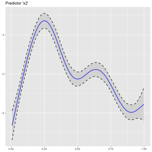
Right now, the only (quick) possibility to plot the smoothing functions of a GAM(M) in R was by using the built-in plot() function. Since I prefer using ggplot2 for all kind of plotting, I implemented the somehow fiddly procedure of plotting GAM smoothing functions using ggplot() in plot_gam():
suppressPackageStartupMessages(library(cowplot)) # for plotting theme
plot_gam(fit_gam, pred = "x2", title = "Predictor 'x2'")
Add odds ratio information into smoothing function plot
So now, we have the odds ratios and we have a plot of the smoothing function. Why not combine both? We can do so using insert_or()! Its main arguments are (i) a ggplot plotting object containing the smooth function (from plot_gam()) and a data frame returned from or_gam() containing information about the predictor and the respective values we want to insert.
plot_object <- plot_gam(fit_gam, pred = "x2", title = "Predictor 'x2'")
or_object1 <- or_gam(data = dat, model = fit_gam, pred = "x2",
  values = c(0.099, 0.198))

# insert first odds ratios into plot
plot_object <- insert_or(plot_object, or_object1, or_yloc = 3,
  values_xloc = 0.04, line_size = 0.5,
  line_type = "dotdash", text_size = 5,
  values_yloc = 0.5, arrow_col = "red")
The odds ratio information is always centered between the two vertical lines. Hence it only looks nice if the gap between the two chosen values (here 0.099 and 0.198) is large enough. If the smoothing line crosses your inserted text, you can correct it by adjusting or_yloc. This argument sets the y-location of the inserted odds ratio information. Depending on the number of digits of your chosen values (here 3), you might also need to adjust the x-axis location of the two values so that these do not interfer with the vertical line.
Let’s add another odds ratio into this plot! This time we simply take the already produced plot as an input to insert_or() and use a new odds ratio object:
or_object2 <- or_gam(data = dat, model = fit_gam, pred = "x2",
  values = c(0.4, 0.6))

# add or_object2 into plot
insert_or(plot_object, or_object2, or_yloc = 2.1, values_yloc = 2,
  line_col = "green4", text_col = "black",
  rect_col = "green4", rect_alpha = 0.2,
  line_alpha = 1, line_type = "dashed",
  arrow_xloc_r = 0.01, arrow_xloc_l = -0.01,
  arrow_length = 0.01, rect = TRUE)
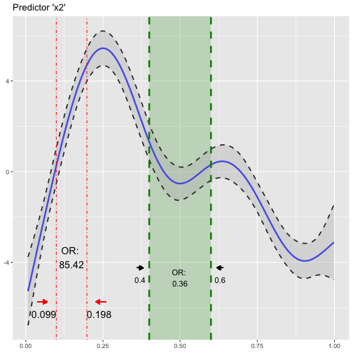
Quite some adjustments were made for this insertion: I adjusted values_yloc because we have only one digit this time. Also, or_yloc was set to a lower value than in the first example to avoid an interference with the smoothing function. A green shaded rectangle was added using rect = TRUE and I set the arrow color to black. Length and position of the arrows very slightly modified using arrow_length, arrow_xloc_r and arrow_xloc_l. If you do not like arrows, simply turn them off using arrow = FALSE. The same logic applies to the shaded rectangle rect = FALSE and the inserted values values = FALSE.
Installation
You can install the package from CRAN by
install.packages("oddsratio")
or from Github using
remotes::install_github("pat-s/oddsratio", build_vignettes = TRUE)